NILE

The NILE estimator can be used to estimate a nonlinear causal influence of a single predictor X on a real-valued response Y. It exploits an instrumental variable (IV) setting with a single exogenous variable A which serves as instrument. Predictions obtained from the NILE estimator are causal predictions in the sense that they predict the values of Y under interventions which break the dependence between X and possible confounders of (X, Y). For further details refer to the paper Christiansen et al. (2020 https://arxiv.org/abs/2006.07433).

Installation

You can install the the development version from GitHub with:

# install.packages("devtools")
devtools::install_github("runesen/NILE")

Example

This is a basic example which shows the idea behind NILE. Let us start by importing the NILE library.

library(NILE)
library(splines)

Suppose that the true (unknown) functional relationship between X and Y is defined by a spline that linearly extrapolates outside the training data.

# true (unknown) functional relationship X -> Y
# (linearly extrapolating beyond "extrap")
fX <- function(x, extrap, beta){
  bx <- splines::ns(x, knots = seq(from=extrap[1], to=extrap[2],
                                   length.out=(n.splines.true+1))[
                                     -c(1,n.splines.true+1)],
                    Boundary.knots = extrap)
  bx%*%beta
}

Let us define the data generating model.

# data generating model
n <- 200
n.splines.true <- 4
set.seed(2)
beta0 <- runif(n.splines.true, -1,1)
alphaA <- alphaEps <- alphaH <- 1/sqrt(3)
A <- runif(n,-1,1)
H <- runif(n,-1,1)
X <- alphaA*A + alphaH*H + alphaEps*runif(n,-1,1)
Y <- fX(x=X,extrap=c(-.7,.7), beta=beta0) + .3*H + .2*runif(n,-1,1)

x.new <- seq(-2,2,length.out=100)
f.new <- fX(x=x.new,extrap=c(-.7,.7), beta=beta0)
plot(X,Y, pch=20)
lines(x.new,f.new,col="#0072B2",lwd=3)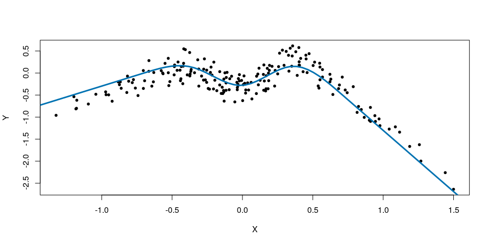

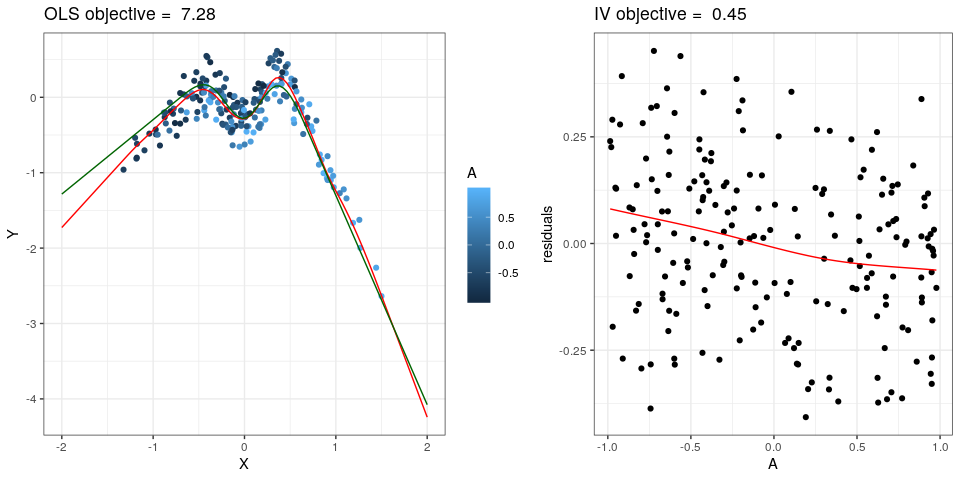
Given the observed dataset, let us now fit NILE.

fit <- NILE(Y, # response
            X, # predictors (so far, only 1-dim supported)
            A, # anchors (1 or 2-dim, although 2-dim is experimental so far)
            lambda.star = "test", # (0 = OLS, Inf = IV, (0,Inf) =
            # nonlinear anchor regression, "test" = NILE)
            test = "tsls.over.ols",
            intercept = TRUE,
            df = 50, # number of splines used for X -> Y
            p.min = 0.05, # level at which test for lambda is performed
            x.new = x.new, # values at which predictions are required
            plot=TRUE, # diagnostics plots
            f.true = function(x) fX(x,c(-.7,.7), beta0), # if supplied, the
            # true causal function is added to the plot
            par.x = list(lambda=NULL, # positive smoothness penalty for X -> Y,
                         # if NULL, it is chosen by CV to minimize out-of-sample
                         # AR objective
                         breaks=NULL, # if breaks are supplied, exactly these
                         # will be used for splines basis
                         num.breaks=20, # will result in num.breaks+2 splines,
                         # ignored if breaks is supplied.
                         n.order=4 # order of splines
                         ),
            par.a = list(lambda=NULL, # positive smoothness penalty for fit of
                         # residuals onto A. If NULL, we first compute the OLS
                         # fit of Y onto X,
                                      # and then choose lambdaA by CV to
                         # minimize the out-of-sample MSE for predicting
                         # the OLS residuals
                         breaks=NULL, # same as above
                         num.breaks=4, # same as above
                         n.order=4 # same as above
                         ))
#> [1] "lambda.cv.a =  1.42932324587573"
#> [1] "lambda.cv.x =  0.0015933292003293"
#> [1] "lambda.star.p.uncorr =  1.45538091659546"

References

Christiansen, R., Pfister, N., Jakobsen, M. E., Gnecco, N., & Peters, J. (2020). The difficult task of distribution generalization in nonlinear models.