Overview
This vignette will guide you through reproducing the numerical simulations and figures of Christiansen et al. (2020). Each section is devoted to reproducing each image or simulation. Once NILE is installed, you can export the code in this guide by typing edit(vignette("vgn_reproduce_results")).
Figure 1 - Impossibility plots
library(ggplot2)
library(gridExtra)
library(grid)
theme_set(theme_bw())


join.smoothly <- function(x,x1,x2,f1,f2,f1prime,f2prime){
  y <- c(f1,f2,f1prime,f2prime)
  A <- matrix(c(1,x1,x1^2,x1^3,
                1,x2,x2^2,x2^3,
                0,1,2*x1,3*x1^2,
                0,1,2*x2,3*x2^2), 4,4, byrow=TRUE)
  b <- solve(A,y)
  sapply(x, function(xx) sum(b*(xx^(0:3))))
}

x <- seq(1,2,.01)
# plot(x,join.smoothly(x,0,1,-1,1))

g.global <- function(a) a+1
g.global.prime <- function(a) 1

g <- function(a, supp = c(-1,1), eps = .5, C=5){
  out <- numeric(length(a))
  w.below <- which(a <= min(supp)-eps)
  w.midlow <- which(a > min(supp)-eps & a < min(supp))
  w.within <- which(a >= min(supp) & a <= max(supp))
  w.midup <- which(a > max(supp) & a < max(supp)+eps)
  w.above <- which(a >= max(supp)+eps)
  if(length(w.below)>0) out[w.below] <- out[w.above] <- C
  if(length(w.midlow)>0) out[w.midlow] <- join.smoothly(a[w.midlow],supp[1]-eps,supp[1],C,g.global(supp[1]),0,g.global.prime(supp[2]))
  if(length(w.within)>0) out[w.within] <- g.global(a[w.within])
  if(length(w.midup)>0) out[w.midup] <- join.smoothly(a[w.midup],supp[2], supp[2]+eps,g.global(supp[2]),C, g.global.prime(supp[2]),0)
  if(length(w.above)>0) out[w.above] <- C
  out
}
a <- seq(-2,2,length.out = 1000)
# plot(a,g(a,eps=.5),type="l",lwd=5)

n <- 200
beta <- 1
set.seed(1)
# observational
A <- runif(n,-1,1)
H <- rnorm(n)
X <- g(A, eps=.5, C=5) + H + .5*rnorm(n)
Y <- beta*X + H + .5*rnorm(n)

bOLS <- lm(Y~X)$coefficients

# interventional
Ai <- rep(1.5,n)
Hi <- rnorm(n)
Xi <- g(Ai, eps=.5, C=5) + Hi + .5*rnorm(n)
Yi <- beta*Xi + Hi + .5*rnorm(n)

df <- data.frame(X=c(X,Xi), A=c(A,Ai), Y=c(Y,Yi),
                 setting = factor(rep(c("observational", "interventional"), each=n),
                                  levels = c("observational", "interventional")))
x.seq <- seq(min(df$X), max(df$X), length.out = 100)
df.line <- data.frame(x = rep(x.seq, 2),
                      y = c(bOLS[1] + bOLS[2]*x.seq,
                            x.seq),
                      model = factor(rep(c("candidate", "causal"), each = length(x.seq))))

pXY <- ggplot() +
  geom_point(data=df, aes(X,Y, col=setting, shape = setting), alpha=.7, size=3) +
  scale_color_manual(values = c("black", "red")) +
  geom_line(data=subset(df.line, model == "candidate"), aes(x,y),size=1, col = "blue") +
  geom_line(data=subset(df.line, model == "causal"), aes(x,y),size=1, col = "#009E73", lty = "dashed") +
  annotate(geom = "text", x = -1, y = 5, label = "training data") +
  annotate(geom = "text", x = 5, y = -1, label = "test data") +
  annotate(geom = "text", x = 3, y = 10, label = "candidate model") +
  # annotate(geom = "text", x = 6, y = 1, label = "causal model") +
  annotate(geom = "text", x = 7.5, y = 6.5, label = "f", col = "#009E73") +
  geom_segment(aes(x = -.5, y = 4, xend = 0, yend =2),
               arrow = arrow(length = unit(0.3, "cm"))) +
  geom_segment(aes(x = 5, y = 0, xend = 5, yend = 2),
               arrow = arrow(length = unit(0.3, "cm"))) +
  geom_segment(aes(x = 5, y = 10, xend = 6, yend = 10),
               arrow = arrow(length = unit(0.3, "cm"))) +
  # geom_segment(aes(x = 6, y = 2, xend = 6.6, yend = 6.3),
  #              arrow = arrow(length = unit(0.3, "cm"))) +
  xlab("x") + ylab("y") +
  # geom_abline(intercept = bOLS[1], slope = bOLS[2]) +
  theme(legend.position = "none",
        text = element_text(size=15),
        plot.title = element_text(size = 14, hjust=.5))

a.seq <- seq(-2,2,length.out = 1000)
df.A <- data.frame(a = a.seq, g = g(a.seq))
df.A$seq <- factor(sapply(1:nrow(df.A), function(i) ifelse(df.A$a[i] < -1, 1, ifelse(df.A$a[i] <= 1, 2, 3))))

grid.a <- seq(-.9, .9, .2)
hist.a <- sapply(grid.a, function(g) sum(abs(A-g) < .1))
m <- max(hist.a)
hist.a <- 4*hist.a/m
df.hist <- data.frame(a=c(grid.a, 1.55), h = c(hist.a, 4), data = c(rep("1",length(grid.a)), "2"))

pA <- ggplot(df.A, aes(a,g)) +
  geom_segment(aes(x = 1, y = .8, xend = 1.4, yend = .1),
               arrow = arrow(length = unit(0.3, "cm"))) +
  geom_line(aes(lty = seq), size=1, col = "black") +
  # geom_line(size=1, col = "black") +
  xlab("a") + ylab("") +
  geom_bar(data=df.hist, aes(x=a,y=h,fill=data), alpha=.2, stat = "identity") +
  annotate(geom = "text", x = -1.6, y = 4.5, label = "g") +
  geom_segment(aes(x = -.8, y = 3.5, xend = -1, yend = 3.5),
               arrow = arrow(length = unit(0.3, "cm"), angle = 90)) +
  geom_segment(aes(x = .8, y = 3.5, xend = 1, yend = 3.5),
               arrow = arrow(length = unit(0.3, "cm"), angle = 90)) +
  annotate(geom = "text", x = 0, y = 3.5, label = "training support") +
  annotate(geom = "text", x = .9, y = 1, label = "intervention") +
  scale_fill_manual(values= c("black", "red")) +
  scale_linetype_manual(values = c("dashed", "solid", "dashed")) +
  theme(legend.position = "none",
        text = element_text(size=15),
        plot.title = element_text(size = 14, hjust=.5))

all.A <- arrangeGrob(pA, pXY, ncol = 2,
                     top = textGrob("support-extending interventions on A", gp=gpar(fontsize=15)))

# # grid.arrange(pA, pXY, ncol=2)
#
# pdf("../figures/impossibility_AtoX_nonlinear.pdf", width = 8, height = 3.5)
# grid.arrange(pA, pXY, ncol=2, top = "support-extending interventions on A")
# dev.off()


#######################
## interventions on X
#######################
f.global <- function(x) -x
f.global.prime <- function(x) -1

f <- function(a, supp = c(-1,1), eps = 1, C=c(-5,5)){
  out <- numeric(length(a))
  w.below <- which(a <= min(supp)-eps)
  w.midlow <- which(a > min(supp)-eps & a < min(supp))
  w.within <- which(a >= min(supp) & a <= max(supp))
  w.midup <- which(a > max(supp) & a < max(supp)+eps)
  w.above <- which(a >= max(supp)+eps)
  if(length(w.below)>0) out[w.below] <- C[1]
  if(length(w.midlow)>0) out[w.midlow] <- join.smoothly(a[w.midlow],supp[1]-eps,supp[1],C[1],f.global(supp[1]),20,f.global.prime(supp[2]))
  if(length(w.within)>0) out[w.within] <- f.global(a[w.within])
  if(length(w.midup)>0) out[w.midup] <- join.smoothly(a[w.midup],supp[2],supp[2]+eps,f.global(supp[2]),C[2], f.global.prime(supp[2]),20)
  if(length(w.above)>0) out[w.above] <- C[2]
  out
}
x <- seq(-2,2,length.out = 1000)
# plot(x,f(x,eps=1),type="l",lwd=5)

n <- 200
beta <- 1
set.seed(1)
# observational
A <- runif(n,-1,1)
H <- runif(n,-1,1)
X <- .4*H + .4*A + .2*runif(n,-1,1)
Y <- f(X) + .5*H + .5*rnorm(n)

Ai <- runif(n,-1,1)
Hi <- runif(n,-1,1)
Xi <- runif(n,1.5,2)
Yi <- f(Xi) + Hi + .5*rnorm(n)


df1 <- data.frame(X=c(X,Xi), A=c(A,Ai), Y=c(Y,Yi),
                 setting = factor(rep(c("observational", "interventional"), each=n),
                                  levels = c("observational", "interventional")))
x.seq <- seq(-2,2,length.out = 1000)
df1.line <- data.frame(x = rep(x.seq, 2),
                      y = c(-x.seq, f(x.seq)),
                      model = factor(rep(c("candidate", "causal"), each = length(x.seq))))

pXY1 <- ggplot() +
  geom_point(data=df1, aes(X,Y, col=setting, shape = setting), alpha=.7, size=3) +
  scale_color_manual(values = c("black", "red")) +
  geom_line(data=subset(df1.line, model == "candidate"), aes(x,y),size=1, col = "blue") +
  geom_line(data=subset(df1.line, model == "causal"), aes(x,y),size=1, col = "#009E73", lty = "dashed") +
  annotate(geom = "text", x = 0, y = 3.5, label = "training data") +
  annotate(geom = "text", x = 1, y = 5.5, label = "test data") +
  annotate(geom = "text", x = -1.2, y = 5.5, label = "candidate model") +
  annotate(geom = "text", x = -1.5, y = -1, label = "f", col = "#009E73") +
  ggtitle("support-extending interventions on X") +
  xlab("x") + ylab("y") +
  # annotate(geom = "text", x = 6, y = 1, label = "causal model") +
  geom_segment(aes(x = 0, y = 3, xend = 0, yend = 1.5),
               arrow = arrow(length = unit(0.3, "cm"))) +
  geom_segment(aes(x = 1.2, y = 5, xend = 1.6, yend = 4),
               arrow = arrow(length = unit(0.3, "cm"))) +
  geom_segment(aes(x = -1.2, y = 5, xend = -1.6, yend = 2.5),
               arrow = arrow(length = unit(0.3, "cm"))) +
  geom_segment(aes(x = -.8, y = -5, xend = -1, yend = -5),
               arrow = arrow(length = unit(0.3, "cm"), angle = 90)) +
  geom_segment(aes(x = .8, y = -5, xend = 1, yend = -5),
               arrow = arrow(length = unit(0.3, "cm"), angle = 90)) +
  geom_segment(aes(x = 1.5, y = -5, xend = 2, yend = -5),
               arrow = arrow(length = unit(0.3, "cm"), angle = 90)) +
  geom_segment(aes(x = 2, y = -5, xend = 1.5, yend = -5),
               arrow = arrow(length = unit(0.3, "cm"), angle = 90)) +
  annotate(geom = "text", x = 0, y = -5, label = "training support") +
  coord_cartesian(ylim=c(-5.5,6)) +
  annotate(geom = "text", x = 1.5, y = -3.5, label = "test support") +
  # geom_segment(aes(x = 1, y = -3.5, xend = 1.5, yend = -4),
  #              arrow = arrow(length = unit(0.3, "cm"))) +
  # xlab("x") + ylab("y") +
  # geom_abline(intercept = bOLS[1], slope = bOLS[2]) +
  theme(legend.position = "none",
        text = element_text(size=15),
        plot.title = element_text(size = 14, hjust=.5))

grid.arrange(pXY1, all.A,ncol=2, widths = c(1,2))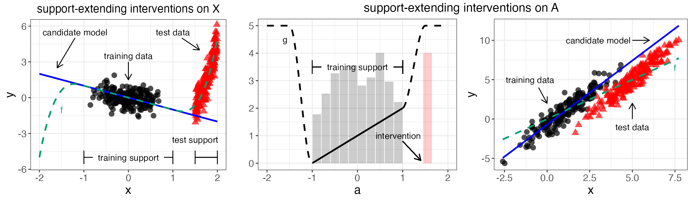
Figure 2 - NILE vs. other methods
library(NILE)
library(R.utils)
library(splines)
library(np)
# X has fixed variance 1/3
n <- 200
fact <- 1 # three times the desired variance of X
df.X <- 50
## missing settings
alphaA <- sqrt(fact/3)
alphaH <- sqrt(2*fact/3)
alphaEps <- 0
## quantiles for different settings
set.seed(1)
N <- 100000
A <- runif(N,-1,1)
H <- runif(N,-1,1)
X <- alphaA*A + alphaH*H + alphaEps*runif(N,-1,1)
q <- quantile(X, probs = c(.05,.95))
qX <- c(-1,1)*(q[2]-q[1])/2
suppX <- c(-1,1)*(alphaA + alphaH + alphaEps)

n.splines.true <- 4
set.seed(4)
beta <- runif(n.splines.true, -1,1)
fX <- function(x=x.new, qx=qX, beta=beta){
  bx <- ns(x, knots = seq(from=qx[1], to=qx[2], length.out=(n.splines.true+1))[-c(1,n.splines.true+1)], Boundary.knots = qx)
  bx%*%beta
}
A <- runif(n,-1,1)
H <- runif(n,-1,1)
X <- alphaA*A + alphaH*H + alphaEps*runif(n,-1,1)
Y <- fX(X,qX,beta) + .3*H + .2*runif(n,-1,1)
x.new <- seq(-2,2,length.out = 100)
f.new <- fX(x.new, qX, beta)
plot(X,Y)
lines(x.new, f.new)

pred.frame <- NULL
k <- 0
Nsim <- 20
for(i in 1:Nsim){
  k <- k+1
  set.seed(k)
  print(paste("sim = ", i))

  A <- runif(n,-1,1)
  H <- runif(n,-1,1)
  X <- alphaA*A + alphaH*H + alphaEps*runif(n,-1,1)
  Y <- fX(X,qX,beta) + .3*H + .2*runif(n,-1,1)

  fit.ols <- tryCatch({withTimeout({NILE(Y=Y,X=X,A=A,lambda.star=0,df=df.X,x.new=x.new,plot=FALSE,par.a=list(lambda=0.1))$pred}, timeout = 180, onTimeout = "error")},
                      error=function(e){
                        print(paste("ERROR OLS: ", e))
                        rep(NA, length(x.new))
                      })

  nile <- tryCatch({withTimeout({NILE(Y=Y,X=X,A=A,lambda.star="test",df=df.X,x.new=x.new,plot=FALSE)}, timeout = 180, onTimeout = "error")},
                   error=function(e){
                     print(paste("ERROR NILE: ", e))
                     list(pred = rep(NA, length(x.new)), lambda.star = NA)
                   })
  fit.nile <- nile$pred
  lambda.star <- nile$lambda.star

  fit.npregiv <- tryCatch({withTimeout({npregiv(y=Y,z=X,w=A,zeval=x.new)$phi.eval}, timeout = 180, onTimeout = "error")},
                          error=function(e){
                            print(paste("ERROR NPREGIV: ", e))
                            rep(NA, length(x.new))
                          })

  pred.frame.loop <- data.frame(x = x.new,
                                fhat = c(fit.ols, fit.nile, fit.npregiv),
                                ftrue = rep(f.new, 3),
                                method = rep(c("OLS", "NILE", "NPREGIV"), each = length(x.new)),
                                lambda.star = lambda.star,
                                alphaA = alphaA,
                                alphaH = alphaH,
                                alphaEps = alphaEps,
                                qXmin = min(qX),
                                qXmax = max(qX),
                                suppXmin = min(suppX),
                                suppXmax = max(suppX),
                                sim = i)
  pred.frame <- rbind(pred.frame, pred.frame.loop)
  write.table(pred.frame, "overlay_estimates_strongconf.txt", quote = FALSE)
}
library(ggplot2)
library(reshape2)
library(gridExtra)
library(R.utils)
library(splines)
library(np)
theme_set(theme_bw())
pred.frame <- read.table("overlay_estimates_strongconf.txt", header = TRUE)

fact <- 1 # three times the desired variance of X
## missing settings
alphaA <- sqrt(1/3)
alphaH <- sqrt(2/3)
alphaEps <- 0
## quantiles for different settings
qX <- c(pred.frame$qXmin[1], pred.frame$qXmax[1])
suppX <- c(pred.frame$suppXmin[1], pred.frame$suppXmax[1])

n.splines.true <- 4
fX <- function(x=x.new, qx=qX, beta=beta){
  bx <- ns(x, knots = seq(from=qx[1], to=qx[2], length.out=(n.splines.true+1))[-c(1,n.splines.true+1)], Boundary.knots = qx)
  bx%*%beta
}

n.plt <- 200
set.seed(4)
beta <- runif(n.splines.true, -1,1)
A1.plt <- runif(n.plt,-1,1)
H1.plt <- runif(n.plt,-1,1)
X1.plt <- alphaA*A1.plt + alphaH*H1.plt + alphaEps*runif(n.plt,-1,1)
Y1.plt <- fX(X1.plt,qX,beta) + .3*H1.plt + .2*runif(n.plt,-1,1)

plt.frame <- data.frame(x=X1.plt, y=Y1.plt)
# ftrue.frame <- data.frame(x=x.pred, ftrue=f.true)

pred.frame$method <- factor(pred.frame$method, levels = c("OLS", "NILE", "NPREGIV"))

p <- ggplot(pred.frame) +
  geom_point(data=plt.frame, aes(x,y), alpha=.5) +
  geom_vline(xintercept = qX, lty = 2) +
  geom_line(aes(x, fhat, col = method, group = sim), size = .2) +
  geom_line(aes(x, ftrue), col = "#009E73", size=1, lty = "dashed") +
  scale_color_manual(values = c("#D55E00","#0072B2", "#CC79A7")) +
  # ggtitle("")
  facet_grid(.~method) +
  coord_cartesian(xlim=c(-2,2), ylim = c(-1, 1)) +
  theme(legend.position = "none")
p


pdf("overlay_estimates.pdf", width = 7, height = 2.5)
p
dev.off()
Figure 3 - Varying confounding
This experiment is computationally intensive, therefore it is advisable to run it in parallel. The number of simulations is 100, so one strategy is to run it in chunks of 10 simulations at a time.
For example, the first chunk of simulations can be run as follows.
SIM <- 1:10
library(NILE)
library(R.utils)
library(splines)
library(np)
# X has fixed variance 1/3
n <- 200
fact <- 1 # three times the desired variance of X
df.X <- 50 # number of splines used
## missing settings
alphaA.seq <- rep(sqrt(fact/3),3)
alphaH.seq <- c(0,sqrt(fact/3),sqrt(2*fact/3))
alphaEps.seq <- sqrt(fact - alphaA.seq^2 - alphaH.seq^2)
## check
alphaA.seq^2 + alphaH.seq^2 + alphaEps.seq^2
## quantiles for different settings
set.seed(1)
n.exp <- length(alphaA.seq)
qX.mat <- sapply(1:n.exp, function(i){
  N <- 100000
  alphaA <- alphaA.seq[i]
  alphaH <- alphaH.seq[i]
  alphaEps <- alphaEps.seq[i]
  A <- runif(N,-1,1)
  H <- runif(N,-1,1)
  X <- alphaA*A + alphaH*H + alphaEps*runif(N,-1,1)
  q <- quantile(X, probs = c(.05,.95))
  c(-1,1)*(q[2]-q[1])/2
})
suppX.mat <- sapply(1:n.exp, function(i){
  alphaA <- alphaA.seq[i]
  alphaH <- alphaH.seq[i]
  alphaEps <- alphaEps.seq[i]
  c(-1,1)*(alphaA + alphaH + alphaEps)
})

n.splines.true <- 4
fX <- function(x, qx, beta){
  bx <- ns(x, knots = seq(from=qx[1], to=qx[2], length.out=(n.splines.true+1))[-c(1,n.splines.true+1)], Boundary.knots = qx)
  bx%*%beta
}

pred.frame <- NULL
meta.frame <- NULL
x.new <- seq(-2,2,length.out = 100)
k <- max(SIM)*n.exp
for(i in SIM){
  for(j in 1:n.exp){
    k <- k+1
    set.seed(k)
    print(paste("sim = ", i, ", alphaseq = ", j))
    alphaA <- alphaA.seq[j]
    alphaEps <- alphaEps.seq[j]
    alphaH <- alphaH.seq[j]
    qX <- qX.mat[,j]
    suppX <- suppX.mat[,j]

    beta <- runif(n.splines.true, -1,1)
    A <- runif(n,-1,1)
    H <- runif(n,-1,1)
    X <- alphaA*A + alphaH*H + alphaEps*runif(n,-1,1)
    Y <- fX(X,qX,beta) + .3*H + .2*runif(n,-1,1)
    f.new <- fX(x.new,qX,beta)

    ols <- tryCatch({
      t1 <- Sys.time()
      res <- withTimeout({NILE(Y=Y,X=X,A=A,lambda.star=0,df=df.X,x.new=x.new,plot=FALSE,par.a=list(lambda=0.1))}, timeout = 180, onTimeout = "silent")
      t2 <- Sys.time()
      if(!is.null(res)){
        out <- list(time = as.numeric(t2-t1),
             fit = res$pred,
             timeout = FALSE,
             error = FALSE)
      }
      if(is.null(res)){
        out <- list(time = 180,
             fit = rep(NA, length(x.new)),
             timeout = TRUE,
             error = FALSE)
      }
      out
    },
    error=function(e){
      print(paste("ERROR OLS: ", e))
      list(time = NA, fit = rep(NA, length(x.new)), timeout = NA, error = TRUE)
    })

    nile <- tryCatch({
      t1 <- Sys.time()
      res <- withTimeout({NILE(Y=Y,X=X,A=A,lambda.star="test",df=df.X,x.new=x.new,plot=FALSE)}, timeout = 180, onTimeout = "silent")
      t2 <- Sys.time()
      if(!is.null(res)){
        out <- list(time = as.numeric(t2-t1),
             lambda = res$lambda.star,
             fit = res$pred,
             timeout = FALSE,
             error = FALSE)
      }
      if(is.null(res)){
        out <- list(time = 180,
             lambda = NA,
             fit = rep(NA, length(x.new)),
             timeout = TRUE,
             error = FALSE)
      }
      out
    },
    error=function(e){
      print(paste("ERROR NILE: ", e))
      list(time = NA, lambda = NA, fit = rep(NA, length(x.new)), timeout = NA, error = TRUE)
    })

    npregiv <- tryCatch({
      t1 <- Sys.time()
      res <- withTimeout({npregiv(y=Y,z=X,w=A,zeval=x.new)}, timeout = 180, onTimeout = "silent")
      t2 <- Sys.time()
      if(!is.null(res)){
        out <- list(time = as.numeric(t2-t1),
             fit = res$phi.eval,
             timeout = FALSE,
             error = FALSE)
      }
      if(is.null(res)){
        out <- list(time = 180,
             fit = rep(NA, length(x.new)),
             timeout = TRUE,
             error = FALSE)
      }
      out
    },
    error=function(e){
      print(paste("ERROR OLS: ", e))
      list(time = NA, fit = rep(NA, length(x.new)), timeout = NA, error = TRUE)
    })

    meta.frame.loop <- data.frame(method = c("OLS", "NILE", "NPREGIV"),
                                  time = c(ols$time, nile$time, npregiv$time),
                                  timeout = c(ols$timeout, nile$timeout, npregiv$timeout),
                                  error = c(ols$error, nile$error, npregiv$error),
                                  lambda.star = nile$lambda,
                                  alphaA = alphaA,
                                  alphaH = alphaH,
                                  alphaEps = alphaEps,
                                  qXmin = min(qX),
                                  qXmax = max(qX),
                                  suppXmin = min(suppX),
                                  suppXmax = max(suppX),
                                  experiment = j,
                                  sim = i)
    meta.frame <- rbind(meta.frame, meta.frame.loop)

    pred.frame.loop <- data.frame(x = x.new,
                                  fhat = c(ols$fit, nile$fit, npregiv$fit),
                                  ftrue = rep(f.new, 3),
                                  method = rep(c("OLS", "NILE", "NPREGIV"), each = length(x.new)),
                                  lambda.star = nile$lambda,
                                  alphaA = alphaA,
                                  alphaH = alphaH,
                                  alphaEps = alphaEps,
                                  qXmin = min(qX),
                                  qXmax = max(qX),
                                  suppXmin = min(suppX),
                                  suppXmax = max(suppX),
                                  experiment = j,
                                  sim = i)
    pred.frame <- rbind(pred.frame, pred.frame.loop)

    write.table(meta.frame, paste0("varying_confounding_meta", min(SIM), ".txt"), quote = FALSE)
    write.table(pred.frame, paste0("varying_confounding_fit", min(SIM), ".txt"), quote = FALSE)
  }
}
Once the results are saved as .txt files, you can produce the plots as follows.
library(ggplot2)
library(reshape2)
library(gridExtra)
theme_set(theme_bw())
pred.frame <- rbind(read.table("varying_confounding_fit1.txt", header = TRUE),
                    read.table("varying_confounding_fit11.txt", header = TRUE),
                    read.table("varying_confounding_fit21.txt", header = TRUE),
                    read.table("varying_confounding_fit31.txt", header = TRUE),
                    read.table("varying_confounding_fit41.txt", header = TRUE),
                    read.table("varying_confounding_fit51.txt", header = TRUE),
                    read.table("varying_confounding_fit61.txt", header = TRUE),
                    read.table("varying_confounding_fit71.txt", header = TRUE),
                    read.table("varying_confounding_fit81.txt", header = TRUE),
                    read.table("varying_confounding_fit91.txt", header = TRUE))

## avg lambdastar
df.summary <- aggregate(lambda.star ~ experiment, pred.frame, mean, na.rm=1)
##
n <- nrow(pred.frame)
n.x <- length(unique(pred.frame$x))
n.m <- length(unique(pred.frame$method))
n.sim <- length(unique(pred.frame$sim))
n.exp <- n/(n.x*n.m*n.sim)

var_xi_Y <- (1/3)*(.3^2+.2^2)

# pred.frame <- subset(pred.frame, method != "IV")
pred.frame$sq.err <- (pred.frame$fhat-pred.frame$ftrue)^2
pred.frame$x.abs <- round(abs(pred.frame$x),2)
pred.frame$alphaA <- round(pred.frame$alphaA,3)
pred.frame$alphaH <- round(pred.frame$alphaH,3)
pred.frame$alphaEps <- round(pred.frame$alphaEps,3)
pred.frame$qXmax <- round(pred.frame$qXmax,3)
pred.frame$lambda.star <- round(pred.frame$lambda.star,3)
error.frame.x.abs <- aggregate(sq.err ~ method + alphaH + qXmax + x.abs + sim, pred.frame, mean)
error.frame.x.abs <- error.frame.x.abs[order(error.frame.x.abs$method, error.frame.x.abs$alphaH, error.frame.x.abs$sim),]
n.x.abs <- length(unique(error.frame.x.abs$x.abs))
error.frame.x.abs$worst.case.mse <- sapply(1:nrow(error.frame.x.abs), function(i) max(error.frame.x.abs$sq.err[(1+floor((i-1)/n.x.abs)*n.x.abs):i])) + var_xi_Y
# error.frame.x.abs$method <- factor(error.frame.x.abs$method,
#                                    levels = c("OLS", "NILE", "NPREGIV", "ORACLE"))
error.frame.x.abs$alphaH <- factor(error.frame.x.abs$alphaH,
                                       levels = sort(unique(error.frame.x.abs$alphaH)),
                                       labels = c(expression(paste("(", alpha[A], ",", alpha[H], ",", alpha[epsilon], ")  =  (", sqrt(1/3),",", 0,",", sqrt(2/3), ")")),
                                                  expression(paste("(", alpha[A],",", alpha[H],",", alpha[epsilon], ")  =  (", sqrt(1/3),",", sqrt(1/3),",", sqrt(1/3), ")")),
                                                  expression(paste("(", alpha[A], ",",alpha[H],",", alpha[epsilon], ")  =  (", sqrt(1/3),",", sqrt(2/3),",", 0, ")"))))

error.frame.x.abs.avg <- aggregate(worst.case.mse ~ method + alphaH + qXmax + x.abs, error.frame.x.abs, mean)
tmp <- subset(error.frame.x.abs.avg, method == "OLS")
tmp$worst.case.mse <- var_xi_Y
tmp$method <- "ORACLE"
error.frame.x.abs.avg <- rbind(error.frame.x.abs.avg, tmp)

error.frame.x.abs.avg$sim <- max(error.frame.x.abs$sim+1)
error.frame.x.abs.avg$sq.err <- NA
error.frame.x.abs.avg$avg <- TRUE
error.frame.x.abs$avg <- FALSE
error.frame.x.abs <- rbind(error.frame.x.abs, error.frame.x.abs.avg)

error.frame.x.abs$method <- factor(error.frame.x.abs$method,
                                   levels = c("OLS", "NILE", "NPREGIV", "ORACLE"))

qX.frame <- subset(error.frame.x.abs.avg, method == "OLS" & x.abs == 2)
rects1 <- qX.frame
rects1$xstart <- 0
rects1$xend <- rects1$qXmax
rects2 <- qX.frame
rects2$xstart <- rects2$qXmax
rects2$xend <- 2
rects <- rbind(rects1, rects2)
rects$col <- factor(rep(1:2, each=n.exp))

#############
## plotting
#############

p <- ggplot() +
  # geom_density(data=df.plt, aes(x=x.plt),alpha=.5) +
  geom_rect(data = rects, aes(xmin = xstart, xmax = xend, ymin = -Inf, ymax = Inf, fill=col), alpha=.1) +
  geom_line(data=error.frame.x.abs, aes(x.abs, worst.case.mse, col=method, lty = method, group = interaction(method,sim,avg), alpha=avg, size = avg)) +
  #geom_line(data=error.frame.x.abs.avg, aes(x.abs, worst.case.mse, col=method, lty = method), size=1) +
  # facet_wrap(. ~ alphaA + alphaH + alphaEps, ncol=5) +
  # geom_vline(aes(xintercept = qXmax),lty=2) +
  # geom_hline(yintercept = var_xi_Y,lty=2, col = "black") +
  facet_grid(. ~ alphaH, labeller = label_parsed) +
  # ggtitle(expression(paste("constant instrument strength alpha_A = ", 1/sqrt(3)))) +
  # ggtitle(expression(paste("constant instrument strength ", alpha[A], " = ", sqrt(1/3)))) +
  # gtitle("generalization performance for different confounding strength") +
  scale_size_manual(values = c(.2, 1)) +
  scale_alpha_manual(values = c(.2, 1)) +
  scale_color_manual(values = c("#D55E00",
                                #"#0072B2",
                                "#0072B2", "#CC79A7", "#009E73")) +
  scale_linetype_manual(values = c(rep("solid",3), "dashed")) +
  scale_fill_manual(values = c("black", "transparent")) +
  coord_cartesian(xlim = c(0,2), ylim = c(0,.3)) +
  xlab("generalization to interventions up to strength") + ylab("worst-case MSE")  +
  theme(plot.title = element_text(hjust=0.5),
        #legend.position = "none",
        legend.background = element_rect(fill = "transparent", colour = NA),
        legend.key = element_rect(fill = "transparent", colour = NA)) +
  guides(fill="none", lty= "none", size = "none", alpha = "none")
p


pdf("varying_confounding_with_variability.pdf", width = 8, height = 2.5)
p
dev.off()
Figure 4 - Varying instrument
This experiment is computationally intensive, therefore it is advisable to run it in parallel. The number of simulations is 100, so one strategy is to run it in chunks of 10 simulations at a time.
For example, the first chunk of simulations can be run as follows.
SIM <- 1:10
library(NILE)
library(R.utils)
library(splines)
library(np)
# X has fixed variance 1/3
n <- 200
fact <- 1 # three times the desired variance of X
df.X <- 50
## missing settings
alphaA.seq <- sqrt(seq(0,2/3,length.out=5))
alphaH.seq <- rep(sqrt(fact/3),5)
alphaEps.seq <- sqrt(fact - alphaA.seq^2 - alphaH.seq^2)
## check
alphaA.seq^2 + alphaH.seq^2 + alphaEps.seq^2
## quantiles for different settings
set.seed(1)
n.exp <- length(alphaA.seq)
qX.mat <- sapply(1:n.exp, function(i){
  N <- 100000
  alphaA <- alphaA.seq[i]
  alphaH <- alphaH.seq[i]
  alphaEps <- alphaEps.seq[i]
  A <- runif(N,-1,1)
  H <- runif(N,-1,1)
  X <- alphaA*A + alphaH*H + alphaEps*runif(N,-1,1)
  q <- quantile(X, probs = c(.05,.95))
  c(-1,1)*(q[2]-q[1])/2
})
suppX.mat <- sapply(1:n.exp, function(i){
  alphaA <- alphaA.seq[i]
  alphaH <- alphaH.seq[i]
  alphaEps <- alphaEps.seq[i]
  c(-1,1)*(alphaA + alphaH + alphaEps)
})

n.splines.true <- 4
fX <- function(x, qx, beta){
  bx <- ns(x, knots = seq(from=qx[1], to=qx[2], length.out=(n.splines.true+1))[-c(1,n.splines.true+1)], Boundary.knots = qx)
  bx%*%beta
}

pred.frame <- NULL
meta.frame <- NULL
x.new <- seq(-2,2,length.out = 100)
k <- max(SIM)*n.exp
for(i in SIM){
  for(j in 1:n.exp){
    k <- k+1
    set.seed(k)
    print(paste("sim = ", i, ", alphaseq = ", j))
    alphaA <- alphaA.seq[j]
    alphaEps <- alphaEps.seq[j]
    alphaH <- alphaH.seq[j]
    qX <- qX.mat[,j]
    suppX <- suppX.mat[,j]

    beta <- runif(n.splines.true, -1,1)
    A <- runif(n,-1,1)
    H <- runif(n,-1,1)
    X <- alphaA*A + alphaH*H + alphaEps*runif(n,-1,1)
    Y <- fX(X,qX,beta) + .3*H + .2*runif(n,-1,1)
    f.new <- fX(x.new,qX,beta)

    ols <- tryCatch({
      t1 <- Sys.time()
      res <- withTimeout({NILE(Y=Y,X=X,A=A,lambda.star=0,df=df.X,x.new=x.new,plot=FALSE,par.a=list(lambda=0.1))}, timeout = 180, onTimeout = "silent")
      t2 <- Sys.time()
      if(!is.null(res)){
        out <- list(time = as.numeric(t2-t1),
                    fit = res$pred,
                    timeout = FALSE,
                    error = FALSE)
      }
      if(is.null(res)){
        out <- list(time = 180,
                    fit = rep(NA, length(x.new)),
                    timeout = TRUE,
                    error = FALSE)
      }
      out
    },
    error=function(e){
      print(paste("ERROR OLS: ", e))
      list(time = NA, fit = rep(NA, length(x.new)), timeout = NA, error = TRUE)
    })

    nile <- tryCatch({
      t1 <- Sys.time()
      res <- withTimeout({NILE(Y=Y,X=X,A=A,lambda.star="test",df=df.X,x.new=x.new,plot=FALSE)}, timeout = 180, onTimeout = "silent")
      t2 <- Sys.time()
      if(!is.null(res)){
        out <- list(time = as.numeric(t2-t1),
                    lambda = res$lambda.star,
                    fit = res$pred,
                    timeout = FALSE,
                    error = FALSE)
      }
      if(is.null(res)){
        out <- list(time = 180,
                    lambda = NA,
                    fit = rep(NA, length(x.new)),
                    timeout = TRUE,
                    error = FALSE)
      }
      out
    },
    error=function(e){
      print(paste("ERROR NILE: ", e))
      list(time = NA, lambda = NA, fit = rep(NA, length(x.new)), timeout = NA, error = TRUE)
    })

    npregiv <- tryCatch({
      t1 <- Sys.time()
      res <- withTimeout({npregiv(y=Y,z=X,w=A,zeval=x.new)}, timeout = 180, onTimeout = "silent")
      t2 <- Sys.time()
      if(!is.null(res)){
        out <- list(time = as.numeric(t2-t1),
                    fit = res$phi.eval,
                    timeout = FALSE,
                    error = FALSE)
      }
      if(is.null(res)){
        out <- list(time = 180,
                    fit = rep(NA, length(x.new)),
                    timeout = TRUE,
                    error = FALSE)
      }
      out
    },
    error=function(e){
      print(paste("ERROR OLS: ", e))
      list(time = NA, fit = rep(NA, length(x.new)), timeout = NA, error = TRUE)
    })

    meta.frame.loop <- data.frame(method = c("OLS", "NILE", "NPREGIV"),
                                  time = c(ols$time, nile$time, npregiv$time),
                                  timeout = c(ols$timeout, nile$timeout, npregiv$timeout),
                                  error = c(ols$error, nile$error, npregiv$error),
                                  lambda.star = nile$lambda,
                                  alphaA = alphaA,
                                  alphaH = alphaH,
                                  alphaEps = alphaEps,
                                  qXmin = min(qX),
                                  qXmax = max(qX),
                                  suppXmin = min(suppX),
                                  suppXmax = max(suppX),
                                  experiment = j,
                                  sim = i)
    meta.frame <- rbind(meta.frame, meta.frame.loop)

    pred.frame.loop <- data.frame(x = x.new,
                                  fhat = c(ols$fit, nile$fit, npregiv$fit),
                                  ftrue = rep(f.new, 3),
                                  method = rep(c("OLS", "NILE", "NPREGIV"), each = length(x.new)),
                                  lambda.star = nile$lambda,
                                  alphaA = alphaA,
                                  alphaH = alphaH,
                                  alphaEps = alphaEps,
                                  qXmin = min(qX),
                                  qXmax = max(qX),
                                  suppXmin = min(suppX),
                                  suppXmax = max(suppX),
                                  experiment = j,
                                  sim = i)
    pred.frame <- rbind(pred.frame, pred.frame.loop)

    write.table(meta.frame, paste0("varying_instrument_meta", min(SIM), ".txt"), quote = FALSE)
    write.table(pred.frame, paste0("varying_instrument_fit", min(SIM), ".txt"), quote = FALSE)
  }
}
Once the results are saved as .txt files, you can produce the plots as follows.
library(ggplot2)
library(reshape2)
library(gridExtra)
theme_set(theme_bw())
pred.frame <- rbind(read.table("varying_instrument_fit1.txt", header = TRUE),
                    read.table("varying_instrument_fit11.txt", header = TRUE),
                    read.table("varying_instrument_fit21.txt", header = TRUE),
                    read.table("varying_instrument_fit31.txt", header = TRUE),
                    read.table("varying_instrument_fit41.txt", header = TRUE),
                    read.table("varying_instrument_fit51.txt", header = TRUE),
                    read.table("varying_instrument_fit61.txt", header = TRUE),
                    read.table("varying_instrument_fit71.txt", header = TRUE),
                    read.table("varying_instrument_fit81.txt", header = TRUE),
                    read.table("varying_instrument_fit91.txt", header = TRUE))

pred.frame <- subset(pred.frame, experiment <= 3)

n <- nrow(pred.frame)
n.x <- length(unique(pred.frame$x))
n.m <- length(unique(pred.frame$method))
n.sim <- length(unique(pred.frame$sim))
n.exp <- n/(n.x*n.m*n.sim)

var_xi_Y <- (1/3)*(.3^2+.2^2)

# pred.frame <- subset(pred.frame, method != "IV")
pred.frame$sq.err <- (pred.frame$fhat-pred.frame$ftrue)^2
pred.frame$x.abs <- round(abs(pred.frame$x),2)
pred.frame$alphaA <- round(pred.frame$alphaA,3)
pred.frame$alphaH <- round(pred.frame$alphaH,3)
pred.frame$alphaEps <- round(pred.frame$alphaEps,3)
pred.frame$qXmax <- round(pred.frame$qXmax,3)
pred.frame$lambda.star <- round(pred.frame$lambda.star,3)
error.frame.x.abs <- aggregate(sq.err ~ method + alphaA + qXmax + x.abs + sim, pred.frame, mean)
error.frame.x.abs <- error.frame.x.abs[order(error.frame.x.abs$method, error.frame.x.abs$alphaA, error.frame.x.abs$sim),]
n.x.abs <- length(unique(error.frame.x.abs$x.abs))
error.frame.x.abs$worst.case.mse <- sapply(1:nrow(error.frame.x.abs), function(i) max(error.frame.x.abs$sq.err[(1+floor((i-1)/n.x.abs)*n.x.abs):i])) + var_xi_Y

error.frame.x.abs$alphaA <- factor(error.frame.x.abs$alphaA,
                                   levels = sort(unique(error.frame.x.abs$alphaA)),
                                   labels = c(expression(paste("(", alpha[A], ",", alpha[H], ",", alpha[epsilon], ")  =  (", 0,",", sqrt(1/3),",", sqrt(2/3), ")")),
                                              expression(paste("(", alpha[A],",", alpha[H],",", alpha[epsilon], ")  =  (", sqrt(1/6),",", sqrt(1/3),",", sqrt(1/2), ")")),
                                              expression(paste("(", alpha[A], ",",alpha[H],",", alpha[epsilon], ")  =  (", sqrt(1/3),",", sqrt(1/3),",", sqrt(1/3), ")"))))

error.frame.x.abs.avg <- aggregate(worst.case.mse ~ method + alphaA + qXmax + x.abs, error.frame.x.abs, mean)
tmp <- subset(error.frame.x.abs.avg, method == "OLS")
tmp$worst.case.mse <- var_xi_Y
tmp$method <- "ORACLE"
error.frame.x.abs.avg <- rbind(error.frame.x.abs.avg, tmp)

error.frame.x.abs.avg$sim <- max(error.frame.x.abs$sim+1)
error.frame.x.abs.avg$sq.err <- NA
error.frame.x.abs.avg$avg <- TRUE
error.frame.x.abs$avg <- FALSE
error.frame.x.abs <- rbind(error.frame.x.abs, error.frame.x.abs.avg)

error.frame.x.abs$method <- factor(error.frame.x.abs$method,
                                   levels = c("OLS", "NILE", "NPREGIV", "ORACLE"))


qX.frame <- subset(error.frame.x.abs.avg, method == "OLS" & x.abs == 2)
rects1 <- qX.frame
rects1$xstart <- 0
rects1$xend <- rects1$qXmax
rects2 <- qX.frame
rects2$xstart <- rects2$qXmax
rects2$xend <- 2
rects <- rbind(rects1, rects2)
rects$col <- factor(rep(1:2, each=n.exp))


p <- ggplot() +
  # geom_density(data=df.plt, aes(x=x.plt),alpha=.5) +
  geom_rect(data = rects, aes(xmin = xstart, xmax = xend, ymin = -Inf, ymax = Inf, fill=col), alpha=.1) +
  geom_line(data=error.frame.x.abs, aes(x.abs, worst.case.mse, col=method, lty = method, group = interaction(method,sim,avg), alpha=avg, size = avg)) +
  #geom_line(data=error.frame.x.abs.avg, aes(x.abs, worst.case.mse, col=method, lty = method), size=1) +
  # facet_wrap(. ~ alphaA + alphaH + alphaEps, ncol=5) +
  # geom_vline(aes(xintercept = qXmax),lty=2) +
  # geom_hline(yintercept = var_xi_Y,lty=2, col = "black") +
  facet_grid(. ~ alphaA, labeller = label_parsed) +
  # ggtitle(expression(paste("constant instrument strength alpha_A = ", 1/sqrt(3)))) +
  # ggtitle(expression(paste("constant instrument strength ", alpha[A], " = ", sqrt(1/3)))) +
  # gtitle("generalization performance for different confounding strength") +
  scale_size_manual(values = c(.2, 1)) +
  scale_alpha_manual(values = c(.2, 1)) +
  scale_color_manual(values = c("#D55E00",
                                #"#0072B2",
                                "#0072B2", "#CC79A7", "#009E73")) +
  scale_linetype_manual(values = c(rep("solid",3), "dashed")) +
  scale_fill_manual(values = c("black", "transparent")) +
  coord_cartesian(xlim = c(0,2), ylim = c(0,.3)) +
  xlab("generalization to interventions up to strength") + ylab("worst-case MSE")  +
  theme(plot.title = element_text(hjust=0.5),
        #legend.position = "none",
        legend.background = element_rect(fill = "transparent", colour = NA),
        legend.key = element_rect(fill = "transparent", colour = NA)) +
  guides(fill="none", lty= "none", size = "none", alpha = "none")
p


pdf("varying_instrument_with_variability.pdf", width = 8, height = 2.5)
p
dev.off()
Figure 5 - Sampling causal functions
library(R.utils)
#> Loading required package: R.oo
#> Loading required package: R.methodsS3
#> R.methodsS3 v1.8.1 (2020-08-26 16:20:06 UTC) successfully loaded. See ?R.methodsS3 for help.
#> R.oo v1.24.0 (2020-08-26 16:11:58 UTC) successfully loaded. See ?R.oo for help.
#>
#> Attaching package: 'R.oo'
#> The following object is masked from 'package:R.methodsS3':
#>
#>     throw
#> The following objects are masked from 'package:methods':
#>
#>     getClasses, getMethods
#> The following objects are masked from 'package:base':
#>
#>     attach, detach, load, save
#> R.utils v2.10.1 (2020-08-26 22:50:31 UTC) successfully loaded. See ?R.utils for help.
#>
#> Attaching package: 'R.utils'
#> The following object is masked from 'package:utils':
#>
#>     timestamp
#> The following objects are masked from 'package:base':
#>
#>     cat, commandArgs, getOption, inherits, isOpen, nullfile, parse,
#>     warnings
library(splines)
library(ggplot2)
theme_set(theme_bw())


alphaA <- alphaH <- alphaEps <- 1/sqrt(3)
## quantiles for different settings
set.seed(1)
N <- 100000
A <- runif(N,-1,1)
H <- runif(N,-1,1)
X <- alphaA*A + alphaH*H + alphaEps*runif(N,-1,1)
q <- quantile(X, probs = c(.05,.95))
qX <- c(-1,1)*(q[2]-q[1])/2
suppX <- c(-1,1)*(alphaA + alphaH + alphaEps)

n.splines.true <- 4
fX <- function(x=x.new, qx=qX, beta=beta){
  bx <- ns(x, knots = seq(from=qx[1], to=qx[2], length.out=(n.splines.true+1))[-c(1,n.splines.true+1)], Boundary.knots = qx)
  bx%*%beta
}

x.new <- seq(-2,2,length.out = 100)
n <- 200
Nsim <- 18
df.data <- df.ftrue <- NULL
k <- 0
for(i in 1:Nsim){
  k <- k+1
  set.seed(k)
  beta <- runif(n.splines.true, -1,1)
  A <- runif(n,-1,1)
  H <- runif(n,-1,1)
  X <- alphaA*A + alphaH*H + alphaEps*runif(n,-1,1)
  Y <- fX(X,qX,beta) + .3*H + .2*runif(n,-1,1)

  f.new <- fX(x.new,qX,beta)
  df.data <- rbind(df.data, data.frame(x=X, y=Y, sim = i))
  df.ftrue <- rbind(df.ftrue, data.frame(x=x.new, f=f.new, sim = i))
}

p <- ggplot() +
  geom_point(data=df.data, aes(x,y), alpha = .7) +
  geom_line(data=df.ftrue, aes(x, f), col = "#009E73", size = 1) +
  geom_vline(xintercept = qX, lty=2) +
  facet_wrap(.~sim, nrow=3)
p
Figure 6 - Varying curvature
This experiment is computationally intensive, therefore it is advisable to run it in parallel. The number of simulations is 100, so one strategy is to run it in chunks of 10 simulations at a time.
For example, the first chunk of simulations can be run as follows.
SIM <- 1:10
library(NILE)
library(R.utils)
library(splines)
library(np)
# X has fixed variance 1/3
n <- 200
fact <- 1 # three times the desired variance of X
df.X <- 50
## missing settings
alphaA <- alphaH <- alphaEps <- sqrt(fact/3)
## quantiles for different settings
set.seed(1)
N <- 100000
A <- runif(N,-1,1)
H <- runif(N,-1,1)
X <- alphaA*A + alphaH*H + alphaEps*runif(N,-1,1)
q <- quantile(X, probs = c(.05,.95))
qX <- c(-1,1)*(q[2]-q[1])/2
suppX <- c(-1,1)*(alphaA + alphaH + alphaEps)

n.exp <- 5
curv.max.seq <- seq(0, 4, length.out = n.exp)

n.splines.true <- 4
fX <- function(x, qx, beta, curv){
  wlo <- which(x < qx[1])
  wup <- which(x > qx[2])
  curv.term <- numeric(length(x))
  curv.term[wlo] <- .5*curv[1]*(x[wlo]-qx[1])^2
  curv.term[wup] <- .5*curv[2]*(x[wup]-qx[2])^2
  bx <- ns(x, knots = seq(from=qx[1], to=qx[2], length.out=(n.splines.true+1))[-c(1,n.splines.true+1)], Boundary.knots = qx)
  lin.term <- bx%*%beta
  lin.term + curv.term
}

# curv.max <- .5
# curv <- runif(2,min=-curv.max,max=curv.max)
# beta <- runif(n.splines.true, -1,1)
# x.new <- seq(-2,2,length.out = 100)
# f.new <- fX(x.new,qX,beta,curv)
# plot(x.new, f.new)
# abline(v=qx)

pred.frame <- NULL
x.new <- seq(-2,2,length.out = 100)
k <- max(SIM)*n.exp
for(i in SIM){
  for(j in 1:n.exp){
    k <- k+1
    set.seed(k)
    print(paste("sim = ", i, ", curv.max.seq = ", j))
    curv.max <- curv.max.seq[j]
    curv <- runif(2,min=-curv.max,max=curv.max)
    beta <- runif(n.splines.true, -1,1)
    A <- runif(n,-1,1)
    H <- runif(n,-1,1)
    X <- alphaA*A + alphaH*H + alphaEps*runif(n,-1,1)
    Y <- fX(X,qX,beta,curv) + .3*H + .2*runif(n,-1,1)
    f.new <- fX(x.new,qX,beta,curv)

    # fit.nile <- tryCatch({withTimeout({NILE(Y=Y,X=X,A=A,lambda.star="PULSE",df=df.X,x.new=x.new,plot=FALSE)$pred}, timeout = 180, onTimeout = "error")},
    #                      error=function(e){
    #                        print(paste("ERROR NILE: ", e))
    #                        rep(NA, length(x.new))
    #                      })
    nile <- tryCatch({withTimeout({NILE(Y=Y,X=X,A=A,lambda.star="test",df=df.X,x.new=x.new,plot=FALSE)}, timeout = 180, onTimeout = "error")},
                     error=function(e){
                       print(paste("ERROR NILE: ", e))
                       list(pred = rep(NA, length(x.new)), lambda.star = NA)
                     })
    fit.nile <- nile$pred
    lambda.star <- nile$lambda.star

    fit.ols <- tryCatch({withTimeout({NILE(Y=Y,X=X,A=A,lambda.star=0,df=df.X,x.new=x.new,plot=FALSE,par.a=list(lambda=0.1))$pred}, timeout = 180, onTimeout = "error")},
                        error=function(e){
                          print(paste("ERROR OLS: ", e))
                          rep(NA, length(x.new))
                        })
    fit.iv <- tryCatch({withTimeout({NILE(Y=Y,X=X,A=A,lambda.star=Inf,df=df.X,x.new=x.new,plot=FALSE)$pred}, timeout = 180, onTimeout = "error")},
                       error=function(e){
                         print(paste("ERROR IV: ", e))
                         rep(NA, length(x.new))
                       })
    fit.npregiv <- tryCatch({withTimeout({npregiv(y=Y,z=X,w=A,zeval=x.new)$phi.eval}, timeout = 180, onTimeout = "error")},
                            error=function(e){
                              print(paste("ERROR NPREGIV: ", e))
                              rep(NA, length(x.new))
                            })

    pred.frame.loop <- data.frame(x = x.new,
                                  fhat = c(fit.ols, fit.nile, fit.iv, fit.npregiv),
                                  ftrue = rep(f.new, 4),
                                  method = rep(c("OLS", "NILE", "IV", "NPREGIV"), each = length(x.new)),
                                  lambda.star = lambda.star,
                                  alphaA = alphaA,
                                  alphaH = alphaH,
                                  alphaEps = alphaEps,
                                  qXmin = min(qX),
                                  qXmax = max(qX),
                                  suppXmin = min(suppX),
                                  suppXmax = max(suppX),
                                  curv.max = curv.max,
                                  sim = i)
    pred.frame <- rbind(pred.frame, pred.frame.loop)
    write.table(pred.frame, paste0("nz_curvature_strong", min(SIM), ".txt"), quote = FALSE)
  }
}
Once the results are saved as .txt files, you can produce the plots as follows.
library(ggplot2)
library(reshape2)
library(gridExtra)
theme_set(theme_bw())
pred.frame <- rbind(read.table("nz_curvature_strong1.txt", header = TRUE),
                    read.table("nz_curvature_strong11.txt", header = TRUE),
                    read.table("nz_curvature_strong21.txt", header = TRUE),
                    read.table("nz_curvature_strong31.txt", header = TRUE),
                    read.table("nz_curvature_strong41.txt", header = TRUE),
                    read.table("nz_curvature_strong51.txt", header = TRUE),
                    read.table("nz_curvature_strong61.txt", header = TRUE),
                    read.table("nz_curvature_strong71.txt", header = TRUE),
                    read.table("nz_curvature_strong81.txt", header = TRUE),
                    read.table("nz_curvature_strong91.txt", header = TRUE))

pred.frame <- subset(pred.frame, method != "IV")
n <- nrow(pred.frame)
n.x <- length(unique(pred.frame$x))
n.m <- length(unique(pred.frame$method))
n.sim <- length(unique(pred.frame$sim))
n.exp <- n/(n.x*n.m*n.sim)

var_xi_Y <- (1/3)*(.3^2+.2^2)

# pred.frame <- subset(pred.frame, method != "IV")
pred.frame$sq.err <- (pred.frame$fhat-pred.frame$ftrue)^2
pred.frame$x.abs <- round(abs(pred.frame$x),2)
pred.frame$curv.max <- round(pred.frame$curv.max,1)
error.frame.x.abs <- aggregate(sq.err ~ method + curv.max + qXmax + x.abs + sim, pred.frame, mean)
error.frame.x.abs <- error.frame.x.abs[order(error.frame.x.abs$method, error.frame.x.abs$curv.max, error.frame.x.abs$sim, error.frame.x.abs$x.abs),]
n.x.abs <- length(unique(error.frame.x.abs$x.abs))
error.frame.x.abs$worst.case.mse <- sapply(1:nrow(error.frame.x.abs), function(i) max(error.frame.x.abs$sq.err[(1+floor((i-1)/n.x.abs)*n.x.abs):i])) + var_xi_Y

error.frame.x.abs$curv.max <- factor(error.frame.x.abs$curv.max,
                                         levels = sort(unique(error.frame.x.abs$curv.max)),
                                         labels = sapply(sort(unique(error.frame.x.abs$curv.max)), function(c) paste0("max. curvature = ", c)))

error.frame.x.abs.avg <- aggregate(worst.case.mse ~ method + curv.max + qXmax + x.abs, error.frame.x.abs, mean)
tmp <- subset(error.frame.x.abs.avg, method == "OLS")
tmp$worst.case.mse <- var_xi_Y
tmp$method <- "ORACLE"
error.frame.x.abs.avg <- rbind(error.frame.x.abs.avg, tmp)

error.frame.x.abs.avg$sim <- max(error.frame.x.abs$sim+1)
error.frame.x.abs.avg$sq.err <- NA
error.frame.x.abs.avg$avg <- TRUE
error.frame.x.abs$avg <- FALSE
error.frame.x.abs <- rbind(error.frame.x.abs, error.frame.x.abs.avg)

error.frame.x.abs$method <- factor(error.frame.x.abs$method,
                                   levels = c("OLS", "NILE", "NPREGIV", "ORACLE"))

qX.frame <- subset(error.frame.x.abs.avg, method == "OLS" & x.abs == 2)
rects1 <- qX.frame
rects1$xstart <- 0
rects1$xend <- rects1$qXmax
rects2 <- qX.frame
rects2$xstart <- rects2$qXmax
rects2$xend <- 2
rects <- rbind(rects1, rects2)
rects$col <- factor(rep(1:2, each=n.exp))

p <- ggplot() +
  geom_rect(data = rects, aes(xmin = xstart, xmax = xend, ymin = -Inf, ymax = Inf, fill=col), alpha=.1) +
  geom_line(data=error.frame.x.abs, aes(x.abs, worst.case.mse, col=method, lty = method, group = interaction(method,sim,avg), alpha=avg, size = avg)) +
  facet_grid(. ~ curv.max) +
  scale_size_manual(values = c(.15, .85)) +
  scale_alpha_manual(values = c(.15, .85)) +
  scale_color_manual(values = c("#D55E00",
                                #"#0072B2",
                                "#0072B2", "#CC79A7", "#009E73")) +
  scale_linetype_manual(values = c(rep("solid",3), "dashed")) +
  scale_fill_manual(values = c("black", "transparent")) +
  coord_cartesian(xlim = c(0,2), ylim = c(0,.3)) +
  xlab("generalization to interventions up to strength") + ylab("worst-case MSE")  +
  theme(plot.title = element_text(hjust=0.5),
        #legend.position = "none",
        legend.background = element_rect(fill = "transparent", colour = NA),
        legend.key = element_rect(fill = "transparent", colour = NA)) +
  guides(fill="none", lty= "none", size = "none", alpha = "none")
p


pdf("varying_extrapolation_curvature_with_variability.pdf", width = 10, height = 2.2)
p
dev.off()